Autoencoder + SINDy + Pendulum
One of my friends send me this video, I put it on watch later as usual and it waits too much time there. When I watched it, it right away blew my mind: I download the paper and dove into the topic.
The idea is to recover dynamical equations from multi-dimensional data using an autoencoder network. In a nutshell, you have a movie of a dynamic system and you want to obtain its equations of motion.
The use of neural networks or deep learning for the prediction of dynamics of dynamical systems presents some criticalities, among which problems of generalization outside the training set examples and also a lack of interpretability of the model obtained, due to the great the number of parameters of such models.
Task
The goal is to find a set of equations that can capture the dynamics of the system and that it is at the same time the most simple as possible. The idea of the considered paper is to combine an autoencoder that carries out a reduction in dimensionality of the input and a method called SINDy (Sparse Identification of Nonlinear Dynamics) that can find a dynamic model for the system in the new latent coordinates.
The data that is collected does not always represent the dynamics of the system in the best or simplest way possible representation for which SINDy would fail or identify templates with many parameters. While autoencoders perform dimensional reductions but they don’t ensure that the new variables in latent space will have simple associated dynamics.
It is, therefore, appropriate to use these two methods simultaneously, to correctly identify the dynamic but at the same time have a simple dynamic model.
Methods
Dataset
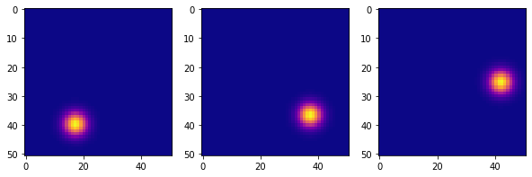
The dataset considered is a collection of snapshots (51x51 images pixel) of a video of a pendulum. The dataset used is generated briefly (more details in the appendix) for which one has a certain freedom in creating the dataset.
We used 100 initial conditions to generate the dataset $ \theta_0 $ and 100 for $ \omega_0 $ by combining them and excluding the initial conditions for which the dynamics of the pendulum is not a cycle limit. Overall, therefore, we have about 5000 initial conditions different, for each of these we have 100 snapshots and each snapshot is a sample with 2601 (51x51) features.
Network architecture
The architecture used is a simple fully connected autoencoder. The autoencoder learns a non-linear representation of the input in a reduced latent space compared to the dimensionality of the samples. The encoder takes as input $ \mathbf{x} (t) \in \mathbb {R} ^ n $ with $ n = 2601 $ and performs a coordinate transformation $ \mathbf {z} (t) = \phi (\mathbf {x} (t)) \in \mathbb {R} ^ d $ where d is the small latent space size. While the decoder performs a transformation $ \tilde {\mathbf {x}} \approx \psi (\mathbf {z}) $ trying to reconstruct the original input. The network consists of:
-
encoder: 3 fully connected layers of 128, 64, 32 neurons
-
a hidden layer made up of a few neurons that acts as a latent space,
-
decoder: 3 layers fully connected inverted with respect to the encoder, therefore 32, 64, 128 neurons.
Sindy: Sparse Identification of Nonlinear Dynamical systems
It is a sparse regression method applied to a library of possibles candidate functions to reconstruct the dynamics of dynamic systems (also non-linear). To build the dynamic model starting from the input data we use a function library and rephrase the problem in the form of regression:
\(\dot {Z} = \mathbf {\Theta} (Z) \mathbf {\Xi}\) The matrix $ \mathbf {\Theta} (Z) $ is constructed by combining candidate functions together: \(\mathbf {\Theta} (Z) = \begin {pmatrix} z_1 (t_0) & z_2 (t_0) & z_3 (t_0) & ... & sin (x_1 (t_0)) & \sqrt {x_2 (t_0)} & ... \\ z_1 (t_1) & ... & ... \\ ... & ... \\ z_1 (t_f) \end {pmatrix}\)
While the unknown matrix $ \mathbf {\Xi} $ contains i
coefficients that determine the active terms of the theta matrix.
Ideally we would like the sparse matrix so that we have few terms
selected from $ \mathbf {\Theta} $. The coefficients $ \xi $ are
updated by the network during training as the $ \omega $ weights of the
net.
\(\mathbf {\Xi} =
\begin {pmatrix}
\xi_ {1,1} & \xi_ {1,2} & \xi_ {1,3} \\
\xi_ {2,1} & ... & ... \\
\xi_ {3,1}
\end {pmatrix}\)
For example, if I wanted to reconstruct the dynamics of the one-dimensional system $ \dot {x} = \sin (x) $ I would have:
\[\dot {X} = \begin {pmatrix} x (t_0) & x ^ 2 (t_0) & \sqrt {x (t_0)} & \sin (x (t_0) & ... \\ x (t_1) & ... & ... \\ ... & ... \\ x (t_f) \end {pmatrix} \begin {pmatrix} 0 \\ 0 \\ 0 \\ 1 \\ ... \\ 0 \end {pmatrix} = \begin {pmatrix} \sin (x (t_0) \\ \sin (x (t_1) \\ \sin (x (t_2) \\ ... \\ ... \\ \sin (x (t_f) \end {pmatrix} = \sin (X)\]Loss
The two methods are combined via the cost function
$ L $; in fact it will not simply be the MSE loss (mean squared loss) between
the autoencoder input $ x $ and the reconstruction $ \tilde {x} $ but they come
added terms that guarantee in addition to the reconstruction of the input,
also the reconstruction of the time derivatives $ \dot {x} $ and $ \dot {z} $ e
finally, a regularization term L1 on the coefficients
$ \mathbf {\Xi} $.
For a dataset with $ m $ samples as input, each loss is defined as
follows:
-
$ L_ {recon} = \frac {1} {m} \sum_ {i = 1} ^ {m} | x_i - \tilde {x_i} | _2 ^ 2 $ measures how well the autoencoder is able to reconstruct the input x.
-
$ L_ {dz} = \frac {1} {m} \sum_ {i = 1} ^ {m} | \dot {z_i} - \Theta (z_i) \mathbf {\Xi} | _2 ^ 2 $ measures how well the model predicts the time derivative correctly of the intrinsic variables $ z $.
-
$ L_ {dx} = \frac {1} {m} \sum_ {i = 1} ^ {m} | \dot {x_i} - \dot {\tilde {x_i}} | _2 ^ 2 $ measures as much as Sindy’s predictions ie $ \dot {\tilde {x}} $ they reconstruct the original input $ \dot {x} $.
-
$ L_ {reg} = \frac {1} {pd} \sum_ {i = 1} ^ {pd} | {\mathbf {\Xi}} | _1 $ is a L1 regularization that promotes the sparsity of the coefficients $ \mathbf {\Xi} $ which coincides with identifying dynamic models simple.
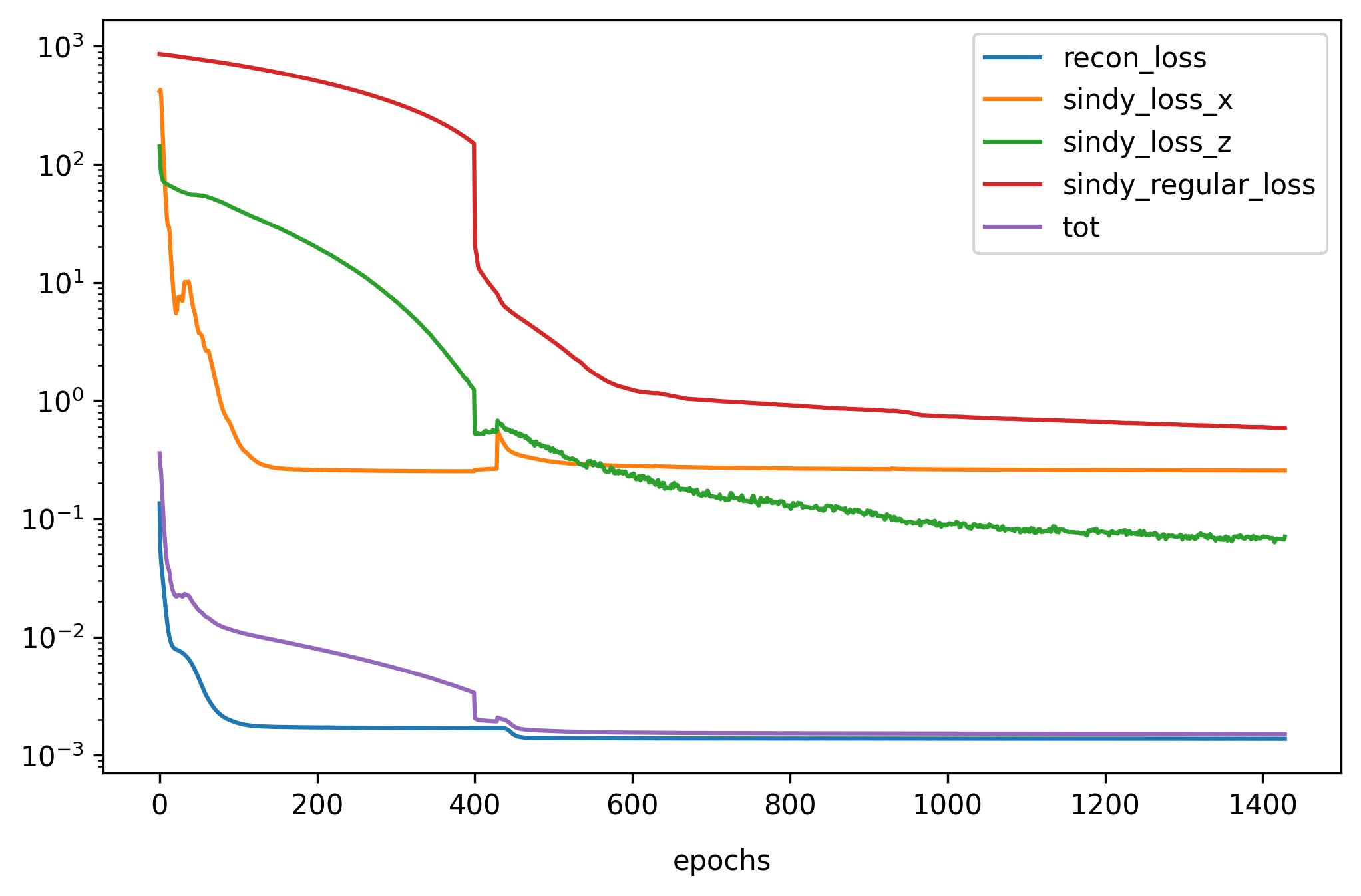
So by combining the four loss terms together with the relative ones hyperparameters the overall loss is the following:
\[L_ {tot} = L_ {recon} + \lambda_1L_ {dx} + \lambda_2L_ {dz} + \lambda_3L_ {reg}\]Results
One of the difficulties during model selection is the lack of a a measure of the accuracy of the dynamics identified, therefore I had to consider the correctness of the coefficients and the parsimoniousness of the dynamic model identified. Not all tested models have identified a plausible dynamic. The best model has found: \(\begin {cases} \dot {z_3} = 0.381 z_8 \\ \dot {z_8} = - 0.672 z_3 \end {cases}\)
Where $ z_3 $ and $ z_8 $ are two of the latent variables extracted from the autoencoder and are the most representative of the dynamic. This is because the other coefficients were null or close to zero and therefore I was able to neglect them. The model identified fails to perfectly recover the initial dynamics of the pendulum but correctly captures its dynamics in the approximation of small angles (linearized model).
! [True and reconstructed attractor] (sindy / attractor.png) {width = “\textwidth”}
Possible future developments
-
Extend to other dynamic systems.
-
Use a convolutional autoencoder as I expect the relevant features of the input are local.
-
Introduce a system of second order time derivatives e then try to rebuild $ \ddot {x} $ from $ x $ directly.
Appendix
For some of you interested in details:
Creation of the synthetic dataset
Recalling the equation of motion of a simple pendulum: \(\ddot {\theta} = - \sin (\theta)\) I can rewrite it as a system of two first-order ODEs, namely:
\[\begin {cases} \dot {\theta} = \omega \\ \dot {\omega} = - \sin (\theta) \end {cases}\]with initial conditions $ \theta_0 $ and $ \omega_0 $ chosen arbitrarily. I have numerically integrated this system from $ t = 0 $ a $ t = $ 5 with an RK4 supplement (Runge-Kutta of the $ 4^o$ order) with a timestep $ dt = 0.05 $. Then to generate the pendulum video I evaluated a 2D Gaussian function on a 51 x 51 point grid.
\[G (x, y, \theta (t)) = \exp (-A [(x - \cos {\theta (t)}) ^ 2 + (y - \sin {\theta (t)}) ^ 2])\]In this way, it is possible to generate how many samples are needed. However, it is important to vary the initial conditions so that the network can have samples of the system at every point of the dynamics.
Propagation of time derivatives
The time derivatives of some appear in the loss function quantities: $ \dot {x} $ we assume to be able to calculate it from the data input, while $ \dot {z} $ and $ \dot {\tilde {x}} $ we must express them in function of known quantities. For example, for $ \dot {z} $:
-
$ m $ number of layers in the network,
-
$ x $ = input,
-
$ z $ = network output,
-
$ I_j = (w_ja_ {j-1} + b_j) $ value of the neurons layer $ j $, so $ \boxed {I_0 = (x \omega_0 + b_0)} $ e $ \boxed {z = I_m = (a_ {m-1} \omega_m + b_m)} $
-
$ a_ {j} (I_j) = f (I_j) $ activation of layer l,
With boundary conditions given by the first layer and by the input: \(\boxed { \frac {dI_0} {dt} = \frac {dI_0} {dx} \frac {dx} {dt} = \dot {x} \; \omega_0 }\)
Applying this rule it is possible to calculate:
-
$ \dot {z} $ knowing $ \dot {x} $,
-
$ \dot {\tilde {x}} $ knowing $ \dot {z} $ (for the latter using the relation $ \dot {z} = \Theta (z) \Xi $, being $ z $ the magnitude Note).
Training Details
I experimented with different combinations by varying the function of activation, the size of the latent space, the algorithm of optimization and initialization of weights. I report the details that led to the best result:
-
Activation function $ f $ = ReLU to avoid phenomena of Vanishing Gradient
-
Optimizer = Adam
-
Initialization of the net weights: extraction from one uniform distribution.
-
The $ \xi $ coefficients have been initialized to $ 1 $.
-
For the choice of the hyperparameters $ \lambda $ in the loss function ho used the values indicated in the paper, respectively: $ \lambda_1 = 5 \times 10 ^ {- 4}, \; \lambda_2 = 5 \times 10 ^ {- 5} $. While for $ \lambda_3 $ I did some tests.
-
Dimension of the latent space $ d = 10 $.
-
The training lasted 1500 epochs (Early Stopping)
-
Batch size = 1024 samples.


Code
If you’re interested take a look at the code implemented on my Github.
References
I based my work on Sindy-Autoencoders architecture of paper from Kathleen Champion et al.